G5AIAI - Introduction to Artificial Intelligence

This course is run at the The University of Nottingham within the School of Computer Science & IT. The course is run by Graham Kendall (EMAIL : gxk@cs.nott.ac.uk)

Blind Searches

Introduction

A blind search (also called an uninformed search) is a search that has no information about its domain. The only thing that a blind search can do is distinguish a non-goal state from a goal state.

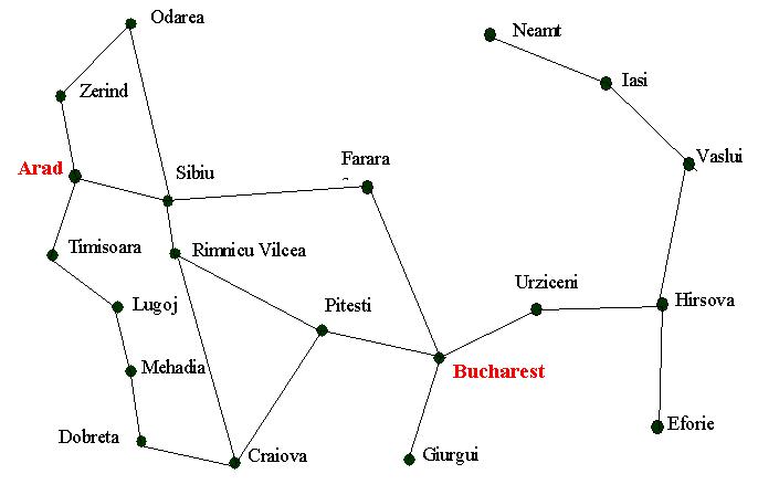
Consider the following, simplified map of Romania

Assume you are currently in Arad and we want to get to Bucharest. If we produce a search tree, level 1 will have three states; Zerind, Sibiu and Timisoara. A blind search will have no preference as to which node it should explore first (later we will see that we can develop search strategies that incorporate some intelligence).

You may wonder why we should use a blind search, when we could use a search with some built in intelligence. The simple answer is that there may not be any information we can use. We might just be looking for an answer and won't know we've found it until we see it.
But it is also useful to study these uninformed searches as they form the basis for some of the intelligent searches that we shall be looking at later.

The blind searches we are about to consider only differ in the order in which we expand the nodes but, as we shall see, this can have a dramatic effect as to how well the search performs.

Breadth-First Search

Using a breadth-first strategy we expand the root level first and then we expand all those nodes (i.e. those at level 1) before we expand any nodes at level 2.
Or to put it another way, all nodes at level d are expanded before any nodes at level d+1.
In fact, if you (as suggested) worked through the search algorithm on the last page (Defining and Implementing a Search) you will have seen a breadth first search in action.
This is because we can implement a breadth first search by using a queuing function that adds expanded nodes to the end of the queue.
Therefore, we could implement a breadth-first search using the following algorithm

Function BREADTH-FIRST-SEARCH(problem) returns a solution or failure
Return GENERAL-SEARCH(problem, ENQUEUE-AT-END)

I have produced a powerpoint presentation to show breadth first search. It might also be worth looking at the powerpoint guidelines I gave you earlier.

We can make the following observations about breadth-first searches
It is a very systematic search strategy as it considers all nodes (states) at level 1 and then all states at level 2 etc.
If there is a solution breadth first search is guaranteed to find it.
If there are several solutions then breadth first search will always find the shallowest goal state first and if the cost of a solution is a non-decreasing function of the depth then it will always find the cheapest solution.

You will recall that we defined four criteria that we are going to use to measure various search strategies; these being completeness, time complexity, space complexity and optimality. In terms of those, breadth-first search is both complete and optimal. Or rather, it is optimal provided that the solution is also the shallowest goal state or, to put it another way, the path cost is a function of the depth.

But what about time and space complexity?

To measure this we have to consider the branching factor, b; that is every state creates b new states.
The root of our tree has 1 state. Level 1 produces b states and the next level produces b² states. The next level produces b³ states.
Assuming the solution is found a level d then the size of the tree is

1 + b + b² + b³ + ... + b^d

(Note : as the solution could be found at any point on the d level then the search tree could be smaller than this).

This type of exponential growth (i.e. O(b^d) ) is not very healthy. You only have to look at the following table to see why.

Depth	Nodes	Time	Memory
0	1	1 millisecond	100 kbytes
2	111	0.1 second	11 kilobytes
4	11,111	11 seconds	1 megabyte
6	10⁶	18 minutes	111 megabytes
8	10⁸	31 hours	11 gigabytes
10	10¹⁰	128 days	1 terabyte
12	10¹²	35 years	111 terabytes
14	10¹⁴	3500 years	11,111 terabytes

Time and memory requirements for breadth-first search, assuming a branching factor of 10, 100 bytes per node and searching 1000 nodes/second

We can make some observations about these figures

Space is more of a factor to breadth first search than time. If you care about the answer you would probably be happy to wait for 31 hours for an answer to a level 8 problem but you are unlikely to have the 11 gigabytes of space that is needed to complete the search.
But time is still an issue. Who has 35 years to wait for an answer to a level 12 problem (or even 128 days to a level 10 problem).
We could argue that as technology gets faster then the type of problems shown above will be solvable. That is true, but even if technology is 100 times faster we would still have to wait 35 years for a level 14 problem and what if we hit a level 15 problem!

It is true to say that breadth first search can only be used for small problems. If we have larger problems to solve then there are better blind search strategies that we can try.

Uniform Cost Search

We have said that breadth first search finds the shallowest goal state and that this will be the cheapest solution so long as the path cost is a function of the depth of the solution. But, if this is not the case, then breadth first search is not guaranteed to find the best (i.e. cheapest) solution.
Uniform cost search remedies this.
It works by always expanding the lowest cost node on the fringe, where the cost is the path cost, g(n). In fact, breadth first search is a uniform cost search with g(n) = DEPTH(n).

Consider the following problem.

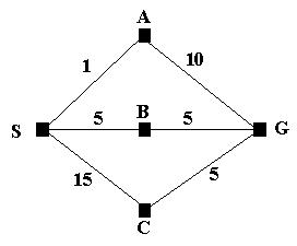
We wish to find the shortest route from S to G; that is S is the initial state and G is the goal state. We can see that SBG is the shortest route but if we let breadth first search loose on the problem it will find the path SAG; assuming that A is the first node to be expanded at level 1.
But this is how uniform cost search tackles the problem.

We start with the initial state and expand it. This leads to the following tree

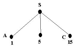
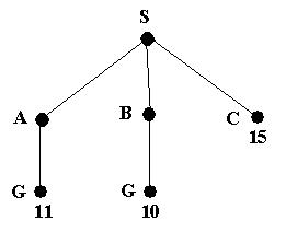
The path cost of A is the cheapest, so it is expanded next; giving the following tree

We now have a goal state but the algorithm does not recognize it yet as there is still a node with a cheaper path cost. In fact, what the algorithm does is order the queue by the path cost so the node with cost 11 will be behind node B in the queue.
Node B (being the cheapest) is now expanded, giving

A goal state (G) will now be at the front of the queue. Therefore the search will end and the path SBG will be returned.

I have produced a powerpoint presentation which shows the above search. It might also be worth looking at the powerpoint guidelines I gave you earlier.

In summary, uniform cost search will find the cheapest solution provided that the cost of the path never decreases as we proceed along the path. If this requirement is not met then we never know when we will meet a negative cost. The result of this would be a need to carry out an exhaustive search of the entire tree.

Depth-First Search

Depth first search explores one branch of a tree before it starts to explore another branch. It can be implemented by adding newly expanded nodes at the front of the queue.

Using the general search algorithm we can implement it as follows.

Function DEPTH-FIRST-SEARCH(problem) returns a solution or failure
Return GENERAL-SEARCH(problem, ENQUEUE-AT-FRONT)

Pictorially, a depth first search can be shown as follows

I have produced a powerpoint presentation to show depth first search. It might also be worth looking at the powerpoint guidelines I gave you earlier.

We can make the following comments about depth first search

It has modest memory requirements. It only needs to store the path from the root to the leaf node as well as the unexpanded nodes. For a state space with a branching factor of b and a maximum depth of m, depth first search requires storage of bm nodes.
The time complexity for depth first search is b^m in the worst case.
If depth first search goes down a infinite branch it will not terminate if it does not find a goal state. If it does find a solution there may be a better solution at a higher level in the tree. Therefore, depth first search is neither complete nor optimal.

Depth-Limited Search

The problem with depth first search is that the search can go down an infinite branch and thus never return.
Depth-limited search avoids this problem by imposing a depth limit which effectively terminates the search at that depth.
The algorithm can be implemented using the general search algorithm by using operators to keep track of the depth.

The choice of the depth parameter can be an important factor. Choosing a parameter that is too deep is wasteful in terms of both time and space. But choosing a depth parameter that is too shallow may result in never reaching a goal state.

As long as the depth parameter, l (this is lower case L, not the digit one), is set "deep enough" then we are guaranteed to find a solution if it exists. Therefore it is complete as long as l >= d (where d is the depth of the solution). If this condition is not met then depth limited search is not complete.

The space requirements for depth limited search are similar to depth first search. That is, O(bl).
The time complexity is O(b^l )

Iterative Deepening Search

The problem with depth limited search is deciding on a suitable depth parameter. If you look at the Romania map you will notice that there are 20 towns. Therefore, any town is reachable from any other town with a maximum path length of 19.
But, closer examination reveals that any town is reachable in at most 9 steps. Therefore, for this problem, the depth parameter should be set as 9. But, of course, this is not always obvious and choosing a parameter is one reason why depth limited searches are avoided.

To overcome this problem there is another search called iterative deepening search.
This search method simply tries all possible depth limits; first 0, then 1, then 2 etc., until a solution is found.
What iterative deepening search is doing is combining breadth first search and depth first search.

I have produced a powerpoint presentation to show iterative deepening search. It might also be worth looking at the powerpoint guidelines I gave you earlier.

It may appear wasteful as it is expanding nodes multiple times. But the overhead is small in comparison to the growth of an exponential search tree.
To show this is the case, consider this.

For a depth limited search to depth d with branching b the number of expansions is

1 + b + b² + … + b^d-2 + b^d-1 + b^d

If we apply some real numbers to this (say b=10 and d=5), we get

1 + 10 + 100 + 1,000 +10,000 + 100,000 = 111,111

For an iterative deepening search the nodes at the bottom level, d, are expanded once, the nodes at d-1 are expanded twice, those at d-3 are expanded three times and so on back to the root.
The formula for this is

(d+1)1 + (d)b+(d-1)b² + … + 3b^d-2 + 2b^d-1 + 1b^d

If we plug in the same numbers we get

6 + 50 + 400 + 3,000 + 20,000 + 100,000 = 123,456

You can see that, compared to the overall number of expansions, the total is not substantially increased.

In fact, when b=10 only about 11% more nodes are expanded for a breadth first search or a depth limited node down to level d.
Even when the branching factor is 2 iterative deepening search only takes about twice as long as a complete breadth first search.

The time complexity for iterative deepening search is O(b^d) with the space complexity being O(bd).

For large search spaces where the depth of the solution is not known iterative deepening search is normally the preferred search method.

Checking for Repeated States

In this section we have looked at five different blind search algorithms. Whilst these algorithms are running it is possible (and for some problems extremely likely) that the same state will be generated more than once.
If we can avoid this then we can limit the number of nodes that are created and, more importantly, stop the need to have to expand the repeated nodes.

There are three methods we can use to stop generating repeated nodes.

Do not generate a node that is the same as the parent node. Or, to put it another way, do not return to the state you have just come from.
Do not create paths with cycles in them. To do this we can check each ancestor node and refuse to create a state that is the same as this set of nodes.
Do not generate any state that is the same as any state generated before. This requires that every state is kept in memory (meaning a potential space complexity of O(b^d)).

The three methods are shown in increasing order of computational overhead in order to implement them.
The last one could be implemented via hash tables to make checking for repeated states as efficient as possible.

Summary

This is a summary of the five search methods that we have looked at. In the following table the following symbols are used.

B = Branching factor
D = Depth of solution
M = Maximum depth of the search tree
L = Depth Limit

Evaluation	Breadth First	Uniform Cost	Depth First	Depth Limited	Iterative Deepening
Time	B^D	B^D	B^M	B^L	B^D
Space	B^D	B^D	BM	BL	BD
Optimal?	Yes	No	No	No	Yes
Complete?	Yes	Yes	No	Yes, ifL>=D	Yes

Last Updated : 27 Sep 2001