
This course is run at the The University of NottinghamĀwithin the School of Computer Science & IT. The course is run by Graham Kendall (EMAIL : gxk@cs.nott.ac.uk)
The powerpoint presentation I gave in the lecture is available for download.
In this part of the course we are going to consider how we can define and implement a search. Following this we will look at some blind search strategies. In addition, you should take a look at the reading list for this part of the course.
If we are going to build a system (write a program) to solve a search problem
we need to do at least two things.
The first of these areas is considered in more detail here. The choice of a search strategy will be considered later.
In order to formulate a problem we can use the following definitions
The Initial State of the problem defines our starting position. For example, in a game of chess the initial state is all the pieces in the usual positions (of course we would have to define this more formally when we wrote our system).
To move from one state to another we apply an Operator. This defines the set of possible actions open to us at a given time. At the start of a chess game we would allow the operators to move the pawns and the knights.
The set of states we can move to from a particular state is often called the Neighbourhood. Another way it is sometimes represented is by applying a Successor Function, S. By applying S(x), where x is the current state, we are returned all states reachable from the current state.
It should be apparent that applying an operator to a state takes us to a new
state.
The initial state and the operators define the State Space of our problem. The
state space is the set of all reachable states from the initial state. In our
chess game, that state space is the set of all valid board configurations as
our operator, from the initial state, should allow us to get to any legal board
configuration.
We need to know when we have solved our problem. A Goal Test, when applied
to the current state, informs us if the current state is a goal state. This
can be explicit, such as the 8-puzzle in a certain board configuration. On other
occasions, there may be more than one condition that represents a solution to
our problem. In the 8-puzzle, for example, we may not care if the numbers go
clockwise, counter-clockwise or in rows or columns; just as long as the numbers
are consecutive.
The goal test can be more abstract. For example, in chess we would not (could
not) enumerate all the possible board configurations which represented checkmate.
Therefore, the goal test would simply check if the king would be taken on the
next move no matter what the opponent does. If this is the case then we have
checkmate.
For some problems we might not only be interested in that we have found a solution
but also in the "cost" of that solution. This is termed the Path Cost
Function and is often denoted by g
In the 8-puzzle the path cost could simply be the number of moves we have made.
If we have another problem where each application of the operator represents
money the path cost could be measured in a financial way.
In some cases, we are not concerned about the path cost. In chess, you may only
be concerned in winning so the path cost is irrelevant as long as the final
position is that your opponent is in checkmate.
In summary, the initial state, the set of operators, the goal states and the
path cost function define a problem.
We could even define a datatype to represent problems; something like
Datatype PROBLEM
Components : INITIAL-STATE, OPERATORS, GOAL-TEST, PATH-COST-FUNCTION
An 8-puzzle can be defined as follows
When we perform a search we want to be able to measure how good it is. This
can be done in a number of ways
Probably the most important is, does it find a solution at all? We are wasting
our time if we implement a search that does not find any sort of solution to
our problem.
It is a good solution? One way of measuring this is to use the path cost. The
lower the path cost the better the solution. We could also take into account
the amount of time the search took and how much memory it used. This is known
as the search cost.
The total cost of the search is given by the path cost added to the search cost.
Another measure we could use is, does it find the optimal solution? For example,
say, we were trying to find the shortest route between two towns. Our search
algorithm might return us a route but is it the cheapest route (by cheapest
we might mean fastest, lowest mileage or routes which avoid suspension bridges
- the choice is yours).
Note, that finding the optimal solution is really just a specialised case of
finding the lowest total cost.
To formalise a little we can define four criteria used to measure search strategies
Later in the course we will be using these measures in order to evaluate different strategies.
Before we look at implementing searches we need to be clear about what a search
tree is.
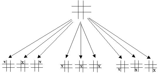
Assume we are just about to start a game of noughts and crosses (or tic tac
toe as the literature often calls it). The board initially looks like this
From this position we can expand the tree to show all possible positions that are reachable from this point. If we assume that the first person to move is playing X then the next level of the tree will look like this
If we expand one of the other nodes we get a tree that looks like this.
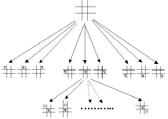
You can see how quickly search trees can grow. This, by anybody's standards, is a very simple game yet at level 2 (assuming the root node is level zero) we have 72 nodes. At the next level we would have 504 nodes. By the next level we have 3024 nodes. And keep in mind this is a very simple game. If we look at something like chess then the search tree gets very large, very quickly.
The way in which a search tree grows is governed by the branching factor. In noughts and crosses the branching factor at level 0 is nine. At the next level it is eight and so on, decreasing by one at each level. The reason chess produces such a large search tree is because it has an average branching factor of 35.
If we use a search tree in order to implement our search strategy then the
search is simply a matter of looking through the search tree in order to find
a goal state for a problem. But as we shall discover this is not as easy as
it sounds.
But before we look at these problems we'll consider how we might implement a
search, in general terms.
First of all we need to decide what information to store at each node of the tree. I suggest the following as a good starting point.
Some of these may seem a bit over the top at the moment but we will make use of all these aspects as we continue our investigations.
Of course, it is possible to define a data structure for these node components
Datatype node
Components: STATE, PARENT-NODE, OPERATOR, DEPTH, PATH-COST
Just so that we are clear. There is a distinction between nodes and states. A node is simply part of a structure that allows us to search our state space. Nodes have parents and depths whereas states do not. It is also possible for two nodes to have the same state which have been arrived at by two different sequences of state changes.
Now we need to decide how best to implement our tree. There is no reason why we cannot simply implement it in a language such as C++ and use the obvious method of having each node with a pointer to its parent node (which would satisfy our need to recognise who our parent is) and a pointer(s) to its children. This is a perfectly reasonable way to proceed but for our purposes it poses two problems.
Firstly, from an implementation point of view we need to implement a tree structure
with varying numbers of children at each node (I refer you to tic tac toe and
I'm sure you can think of many other examples). It's obviously not impossible
but there is an easier way which we'll look at in a moment.
Secondly, as our search proceeds, we need to expand certain nodes of our tree.
The nodes that are candidates for expansion are the leaf nodes of our tree and
they are often called the fringe or frontier nodes. The problem we have is deciding
which node, from the set of fringe nodes, we should expand next.
We could look at every node in our tree (which either means navigating to every
fringe node or maintaining a list) and choosing the best one. But it would be
nice if we always had available the next node that we wish to expand. And we
can do this, as explained below.
If we implement the tree using a queue we can always take the next node from
the head of the queue as the one to expand. Our queue will have the familiar
queue functions; such as
We also need a way of inserting elements into the queue. As we will want to insert elements at different places in the queue, depending on the search strategy we adopt, we will use a function to do this.
Armed with this information we can now define a function that will perform a search.
Function GENERAL-SEARCH(problem, QUEUING-FN) returns a solution or failure
nodes = MAKE-QUEUE(MAKE-NODE(INITIAL-STATE[problem]))
Loop do
If nodes is empty then return failure
node = REMOVE-FRONT(nodes)
If GOAL-TEST[problem] applied to STATE(node) succeeds then return node
nodes = QUEUING-FN(nodes,EXPAND(node,OPERATORS[problem]))
End Loop
End Function
We will be making extensive use of this function as our investigation into search strategies progresses.
For now, assume that the queuing function always adds new nodes to the end of the queue. Work through the algorithm and make sure you understand how it works.
ĀLast Updated : 11 Sep 2001