This course is run at the The University of NottinghamĀwithin the School of Computer Science & IT. The course is run by Graham Kendall (EMAIL : gxk@cs.nott.ac.uk)
The powerpoint presentation I gave in the lecture is available for download.
In this part of the course we are going to consider how we can implement heuristic searches. In addition, you should take a look at the reading list for this part of the course.
The idea behind a heuristic search is that we explore the node that is most
likely to be nearest to a goal state. To do this we use a heuristic function
which tells us how close we are to a goal state.
There is no guarantee that the heuristic function will return a value that ensures
that a particular node is closer to a goal state than any other another node.
If we could do that we would not be carrying out a search. We would simply be
moving through the various states in order to reach the goal state.
To implement a heuristic function we need to have some knowledge of the domain. That is, the heuristic function has to know something about the problem so that it can judge how close the current state is to the goal state.
When we looked at blind searches we have already seen one type of evaluation
function, where we expanded the node with the lowest path cost (for the uniform
cost search).
Using this type of evaluation function we are calculating the cheapest cost
so far. Heuristic searches are different in that we are trying to estimate how
close we are from a goal state, not how cheap the solution is so far.
You might recall that the path cost function is usually denoted by g(n). A heuristic function is normally denoted h(n), that is
h(n) = estimated cost of the cheapest
path from the state at node n to a goal state
To implement a heuristic search we need to order the nodes based on the value
returned from the heuristic function.
We can implement such a search using the general search algorithm. We call the
function BEST-FIRST-SEARCH as the function chooses the best node to expand first.
(In fact, we cannot be sure we are expanding the best node first (otherwise,
it would not be a search at all - just a march from the current state to the
goal state) but, given our current knowledge we believe it to be the best node
- but calling the function BELIEVED-TO-BE-BEST-FIRST-SEARCH is a bit of a mouthful).
Function BEST-FIRST-SEARCH(problem, EVAL-FN) returns a solution sequence
Inputs : problem, a problem
Eval-Fn, an evaluation function
Queueing-Fn = a function that orders nodes by EVAL-FN
Return GENERAL-SEARCH(problem, Queueing-Fn)
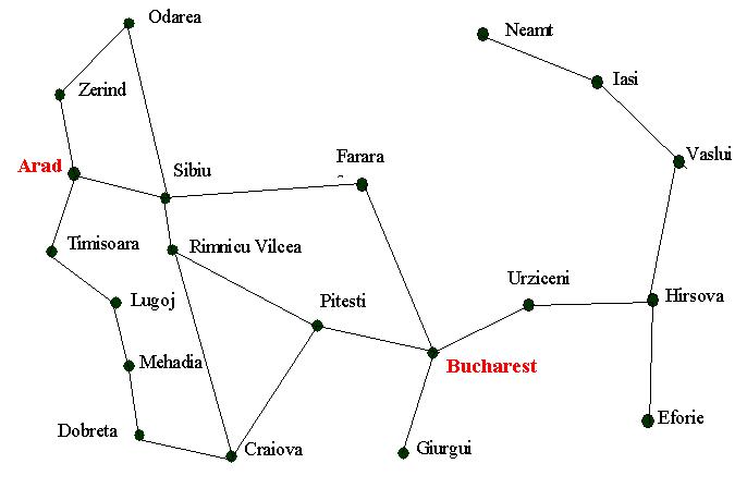
We can develop a heuristic function that helps us to find a solution to the
Romanian route finding problem. One possible heuristic is based on the straight
line distance (as the crow flies) between two cities.
Assume, as before in the blind
search page, that we are trying to get from Arad to Bucharest. Whenever
we find ourselves in a city we look at the neighbouring cites and go to the
one that has the nearest straight line distance (SLD) to Bucharest. We can define
the heuristic function as
hSLD(n) = straight line distance between n and the goal location
Of course, this heuristic might not always give us the best city to go to. Two possible reasons are
But as a general strategy using the SLD heuristic it is a good one to adopt
and is likely to find a solution faster than a blind search.
Greedy search is an implementation of the best search philosophy. It works
on the principle that the largest "bite" is taken from the problem
(and thus the name greedy search).
Greedy search seeks to minimise the estimated cost to reach the goal. To do
this it expands the node that is judged to be closest to the goal state. To
make this judgement is uses the heuristic function, h.
Given an heuristic function h, we can implement a greedy search as follows
Function GREEDY-SEARCH(problem) returns a solution of failure
Return BEST-FIRST-SEARCH(problem,
h)
Given the Arad/Bucharest route finding problem and the hSLD heuristic, greedy search would work as follows (the map has been re-produced below, along with the SLD table)
|
Town
|
SLD to Bucharest
|
| Arad |
366
|
| Bucharest |
0
|
| Craiova |
160
|
| Dobreta |
242
|
| Eforie |
161
|
| Fagaras |
178
|
| Giurgiu |
77
|
| Hirsova |
151
|
| Iasi |
226
|
| Lugoj |
244
|
| Mehadia |
241
|
| Neamt |
234
|
| Oradea |
380
|
| Pitesti |
98
|
| Rimnicu Vilcea |
193
|
| Sibiu |
253
|
| Timisoara |
329
|
| Urziceni |
80
|
| Vaslui |
199
|
| Zerind |
374
|
We start at Arad. This has an SLD of 366 to Bucharest and as it is the only
node we have got, we expand it.
After expanding we have three new nodes (Zerind, Sibiu and Timisoara). These
have SLD's of 374, 253 and 329 respectively. The SLD heuristic tells us that
Sibiu should be expanded next.
This leads to four new nodes (Oradea, Arad, Faragas and Rimnicu Vilcea) with
SLD's of 380, 366, 178 and 193.
Next we choose Faragas to expand as this has the lowest heuristic value. This
step leads to Bucharest being generated which (with a heuristic value of 0)
is a goal state.
If you are unsure as to how this search progresses you might find it useful to draw the search tree.
Using this heuristic led to a very efficient search. We never expanded a node
that was not on the solution path (a minimal search cost).
But, notice that it is not optimal. If we had gone from Sibiu through Rimnicu
Vilcea and Pitesti to Bucharest we would have travelled a shorter distance.
This comes about because we always prefer to take the "biggest bite"
from the problem so we went to Fagaras rather than Rimnicu Vilcea as Faragas
had a shorter SLD even though Rimnicu Vilcea is actually closer.
Or, to put it another way, greedy search is only concerned with short term aims.
It never looks ahead to see what dangers might be lurking.
Having said that, it is true to say, that greedy searches often perform well
although they cannot be guaranteed to give an optimal solution.
And, by looking at the map, we can see one of the problems that we described
above.
If you start at Iasi and were trying to get to Fagaras you would initially go
to Neamt as this is closer to Fagaras than Vaslui. But you would eventually
need to go back through Iasi and through Vaslui to get to your destination.
This example also shows that you may have to check for repeated states. If you
do not then you will forever move between Neamt and Iasi.
As discussed above greedy searches are not optimal. It is also not complete
as we can start down a path and never return (consider the Neamt/Valsui problem
we discussed above). In these respects greedy search is similar to depth first
search. In fact, it is also similar in the way that it explores one path at
a time and then backtracks.
Greedy search has time complexity of O(bm) (where m is the maximum
depth of the search tree). The space complexity is the same as all nodes have
to be kept in memory.
In the above section we considered greedy search. This search method minimises
the cost to the goal using an heuristic function, h(n). Greedy search
can considerably cut the search time but it is neither optimal nor complete.
By comparison uniform cost
search minimises the cost of the path so far, g(n). Uniform
cost search is both optimal and complete but can be very inefficient.
It would be nice if we could combine both these search strategies to get the advantages of both. And we can do that simply by combining both evaluation functions. That is
f(n) = g(n) + h(n)
As g(n) gives the path cost from the start node to node n and h(n) gives the estimated cost of the cheapest path from n to the goal, we have
f(n) = estimated cost of the cheapest solution through n
The good thing about this strategy is that it can be proved to be optimal and complete, given a simple restriction on the h function - which we discuss below.
We can implement A* search as follows
Function A*-SEARCH(problem) returns a solution of failure
Return BEST-FIRST-SEARCH(problem,
g + h)
Note, that if you work through this algorithm by hand (or implement it), you
should always expand the lowest cost node on the fringe, wherever that node
is in the search tree. That is, the nodes you select to expand next are not
just restricted to nodes that have just been generated.
Of course, this is built into the algorithm as the queuing function "automatically"
orders the nodes in this way.
There is a powerpoint presentation which shows the A* search in action, being applied to the map above. This is also the example given in the book, although the powerpoint presentation completes the search, the book just gets you started.
The restriction we mentioned above for the h function is simply this
The h function must never overestimate the cost to reach the goal.
Such an h is called an admissible heuristic.
Another way of describing admissible functions is to say they are optimistic,
as they always think the cost to the goal is less than it actually is.
If we have an admissible h function, this naturally transfers to the f function as f never overestimates the actual cost to the best solution through n.
It is obvious that the SLD heuristic function is admissible as we can never
find a shorter distance between any two towns.
A* is optimal and complete but it is not all good news.
It can be shown that the number of nodes that are searched is still exponential
to length of the search space for most problems. This has implications for the
time of the search but is normally more serious for the space that is required.
So far we have only considered one heuristic function (straight line distance). In this section we consider some other heuristic function and look at some of the properties.
The 8-puzzle, for those of you who don't know, consists of a square of eight tiles and one blank. The aim is to slide the tiles, one at a time to reach a goal state. A typical problem is shown below.
|
5
|
4
|
|
1
|
2
|
3
|
|
6
|
1
|
8
|
8
|
|
4
|
|
7
|
3
|
2
|
7
|
6
|
5
|
|
Initial State
|
Goal State
|
||||
This problem is just the right level that makes it difficult enough to study
yet not so difficult that we quickly get bogged down in its complexity.
A typical solution is about twenty steps. The branching factor is about three
(four when the empty tile is in the middle, two when the empty square is in
a corner and three for other positions).
This means an exhaustive search would look at about 320 states (or
3.5 * 109).
However, by keeping track of repeated states we can reduce this figure to 362,880
as there are only 9! possible arrangements of the tiles.
But, even 362,880 is a lot of states to search (and store) so we should next look for a good heuristic function.
If we want to find an optimal solution we need a heuristic that never over-estimates the number of steps to the goal. That is we need an admissible heuristic.
Here are two possibilities
h1 = the number of tiles that are in the wrong position.
In the above figure (for the initial state) this would return a value of seven,
as seven of the eight tiles are out of position.
This heuristic is clearly admissible as each tile that is out of place needs
to be moved at least once to get it to its correct location.
h2 = the sum of the distances of the tiles from their
goal positions. The method we will use to calculate how far a tile is from its
goal position is to sum the number of horizontal and vertical positions.
This method of calculating distance is sometimes known as the city block distance
or Manhattan distance.
This heuristic function is also admissible as a tile must move at least its
Manhattan distance in order to get to the correct position.
The Manhattan distance for the initial state above is
h2 = 2 + 3 + 3 + 2 + 4 + 2 + 0 + 2 = 18
where the figures given are for tiles 1 through 8.
Of the two 8-puzzle heuristic functions we have developed how do we decide
which one is the best one to use?
One method is to create many instance of the problem and use both heuristic
functions to see which one gives us the best solutions.
The following table shows the results of an averaged 100 runs at depths (solution
length) 2, 4, 6, …, 24 using A* with the h1 and h2
heuristic functions (for comparison we also show the results for a non-heuristic
method; Iterative Deepening Search (IDS) - at least we show it until the numbers
get too large). The search cost figures show the average number of nodes that
were expanded (the EBF figures are explained below).
|
Search Cost
|
EBF
|
|||||
|
Depth
|
IDS
|
A*(h1)
|
A*(h2)
|
IDS
|
A*(h1)
|
A*(h2)
|
| 2 |
10
|
6
|
6
|
2.45
|
1.79
|
1.79
|
| 4 |
112
|
13
|
12
|
2.87
|
1.48
|
1.45
|
| 6 |
680
|
20
|
18
|
2.73
|
1.34
|
1.30
|
| 8 |
6384
|
39
|
25
|
2.80
|
1.33
|
1.24
|
| 10 |
47127
|
93
|
39
|
2.79
|
1.38
|
1.22
|
| 12 |
364404
|
227
|
73
|
2.78
|
1.42
|
1.24
|
| 14 |
3473941
|
539
|
113
|
2.83
|
1.44
|
1.23
|
| 16 |
|
1301
|
211
|
|
1.45
|
1.25
|
| 18 |
|
3056
|
363
|
|
1.46
|
1.26
|
| 20 |
|
7276
|
676
|
|
1.47
|
1.27
|
| 22 |
|
18094
|
1219
|
|
1.48
|
1.28
|
| 24 |
|
39135
|
1641
|
|
1.48
|
1.26
|
From these results it is obvious that h2 is the better heuristic as it results in less nodes being expanded. But, why is this the case?
An obvious reason why more nodes are expanded is the branching factor. If the
branching factor is high then more nodes will be expanded.
Therefore, one way to measure the quality of a heuristic function is to find
out its average branching factor.
If we are using A* search for problem and the solution depth is d, then b* is
the branching factor that a uniform depth d would have to have in order to contain
N nodes. Thus,
N = 1 + b* + (b*)2 + … + (b*)d
To make the example more concrete, if A* finds a solution at depth 5 using 52 nodes then the effective branching factor is 1.91. That is
52 = 1 + 1.91 + (1.91)2 + (1.91)3 + (1.91)4 + (1.91)5
The Effective Branching Factor is shown in the table above for the various
search strategies.
We can see from this that A* using h2 has a lower effective
branching factor and thus h2 is a better heuristic than h1.
We could ask if h2 is always better than h1. In fact, it is easy to see that for any node n, h2(n) => h1(n). This is called domination and we say that h2 dominates h1. And domination translates directly into efficiency.
Inventing Heuristic Functions
It is one thing being able to say that h2 dominates h1 but how
could we come up with h2 (or even h1) in the first place.
Both h1 and h2 are estimates of the number of moves to the final
solution. It is likely that we will need more moves that the estimate (bear
in mind the admissible property). But if we change the rules of the game slightly
then we can make these heuristics give an exact path length needed to solve
the problem.
For example, if the rules were changed so that we could move any tile to the
blank square then h1 would give an exact value as to the path length
required to solve the problem.
Similarly, if a tile could move one square in any direction, even to an occupied
square, then h2 gives an exact path length to the solution.
These changes to the rules are relaxing the rules and a problem that has less
restrictive operators is called a relaxed problem.
It is often the case that the cost of an exact solution to a relaxed problem
is a good heuristic for the original problem.
Below you will find some old exam questions that cover the A* algorithm. You should attempt these questions before you try the self assessment part of this course as you may be asked questions about these exams. Therefore, when you take the self assessment exercise you should have your worked answers to hand.
You should also attempt G5BAIM 1999/2000, question 1(b) and G5AIAI 2000/2001, question 1 and have the worked answers of these to hand (these two questions are only available in Word).
I have supplied a complete set of old exam papers so that you can see the type of questions I have set in the past. The questions also contain answers (though not model answers), including to those above. Of course, it's better if you try the questions without looking at the answers, but that is up to you.
ĀLast Updated : 14 Sep 2001